Stochastic Weight Averaging - Gaussian (SWAG)

%%capture
%pip install git+https://github.com/lightning-uq-box/lightning-uq-box.git

Theoretic Foundation

SWAG is an approximate Bayesian method and uses a low-rank Gaussian distribution as an approximation to the posterior over model parameters. The quality of approximation to the posterior over model parameters is based on using a high SGD learning rate that periodically stores weight parameters in the last few epochs of training Maddox, 2019. SWAG is based on Stochastic Weight Averaging (SWA), as proposed in Izmailov, 2018. For SWA the weights are obtained by minimising the MSE loss with a variant of stochastic gradient descent. After, a number of burn-in epochs, \(\tilde{t} = T-m\), the last \(m\) weights are stored and averaged to obtain an approximation to the posterior, by

\[\theta_{SWA} = \frac{1}{m}\sum_{t=\tilde{t}}^T \theta_t.\]

For SWAG we use the implementation as proposed by Maddox, 2019. Here the posterior is approximated by a Gaussian distribution with the SWA mean and a covariance matrix over the stochastic parameters that consists of a low rank matrix plus a diagonal,

\[p(\theta |D) \approxeq \mathcal{N}\left(\theta_{SWA}, \frac{1}{2}(\Sigma_{diag}+\Sigma_{low-rank})\right).\]

The diagonal part of the covariance is given by

\[\Sigma_{diag} = \text{diag}(\bar{\theta^2} - \theta_{SWA}^2)\]

where,

\[\bar{\theta^2} = \frac{1}{m}\sum_{t=\tilde{t}}^T \theta_t^2.\]

The low rank part of the covariance is given by

\[\Sigma_{low-rank} = \frac{1}{m}\sum_{t=\tilde{t}}^T (\theta_t - \bar{\theta}_t) (\theta_t - \bar{\theta}_t)^T,\]

where \(\bar{\theta}_t\) is the running estimate of the mean of the parameters from the first \(t\) epochs or also samples. In order to approximate the mean prediction, we again resort to sampling from the posterior. With \(\theta_s \sim p(\theta|D)\) for \(s \in \{1, ...,S\}\), the mean prediction is given by

\[\hat{y}(x^{\star}) = \frac{1}{S} \sum_{s=1}^S f_{\theta_s}(x^{\star}),\]

and obtain the predictive uncertainty by

\[\sigma(x^{\star}) = \sqrt{\frac{1}{S} \sum_{s=1}^S f_{\theta_s}(x^{\star})^2 - \hat{y}(x^{\star})^2}.\]

For the subnet strategy, we include selecting the parameters to be stochastic by module names.

Imports

import os

import tempfile
from functools import partial

import matplotlib.pyplot as plt
import torch
import torch.nn as nn
from lightning import Trainer
from lightning.pytorch import seed_everything
from lightning.pytorch.loggers import CSVLogger

from lightning_uq_box.datamodules import ToyHeteroscedasticDatamodule
from lightning_uq_box.models import MLP
from lightning_uq_box.uq_methods import NLL, MVERegression, SWAGRegression
from lightning_uq_box.viz_utils import (
    plot_calibration_uq_toolbox,
    plot_predictions_regression,
    plot_toy_regression_data,
    plot_training_metrics,
)

plt.rcParams["figure.figsize"] = [14, 5]

%load_ext autoreload
%autoreload 2

seed_everything(0)  # seed everything for reproducibility

Seed set to 0

0

We define a temporary directory to look at some training metrics and results.

my_temp_dir = tempfile.mkdtemp()

Datamodule

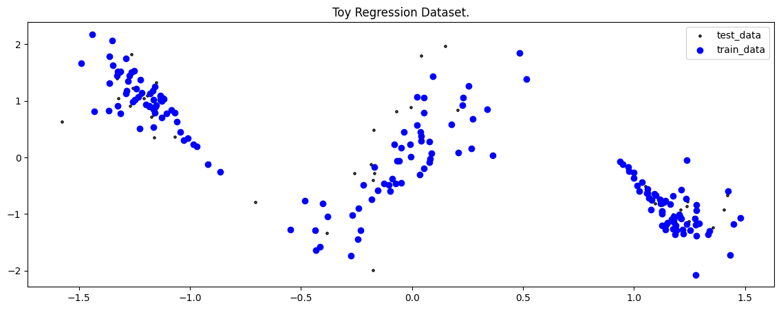
To demonstrate the method, we will make use of a Toy Regression Example that is defined as a Lightning Datamodule. While this might seem like overkill for a small toy problem, we think it is more helpful how the individual pieces of the library fit together so you can train models on more complex tasks.

dm = ToyHeteroscedasticDatamodule()

X_train, Y_train, train_loader, X_test, Y_test, test_loader, X_gtext, Y_gtext = (
    dm.X_train,
    dm.Y_train,
    dm.train_dataloader(),
    dm.X_test,
    dm.Y_test,
    dm.test_dataloader(),
    dm.X_gtext,
    dm.Y_gtext,
)

fig = plot_toy_regression_data(X_train, Y_train, X_test, Y_test)

Model

For our Toy Regression problem, we will use a simple Multi-layer Perceptron (MLP) that you can configure to your needs. For the documentation of the MLP see here. We define a model with two outputs to train with the Negative Log Likelihood.

network = MLP(n_inputs=1, n_hidden=[50, 50, 50], n_outputs=2, activation_fn=nn.Tanh())
network

MLP(
  (model): Sequential(
    (0): Linear(in_features=1, out_features=50, bias=True)
    (1): Tanh()
    (2): Dropout(p=0.0, inplace=False)
    (3): Linear(in_features=50, out_features=50, bias=True)
    (4): Tanh()
    (5): Dropout(p=0.0, inplace=False)
    (6): Linear(in_features=50, out_features=50, bias=True)
    (7): Tanh()
    (8): Dropout(p=0.0, inplace=False)
    (9): Linear(in_features=50, out_features=2, bias=True)
  )
)

With an underlying neural network, we can now use our desired UQ-Method as a sort of wrapper. All UQ-Methods are implemented as LightningModule that allow us to concisely organize the code and remove as much boilerplate code as possible. In the case of SWAG, the method is implemented as a sort of “post-processin” step, where you first train a model with a MAP estimate and subsequently apply SWAG to capture epistemic uncertainty over the neural network weights. Hence, we will first fit a deterministic model, in this case one that outputs the parameters of a Gaussian Distribution and train with the Negative Log Likelihood.

deterministic_model = MVERegression(
    network, burnin_epochs=50, optimizer=partial(torch.optim.Adam, lr=1e-3)
)

Trainer

Now that we have a LightningDataModule and a UQ-Method as a LightningModule, we can conduct training with a Lightning Trainer. It has tons of options to make your life easier, so we encourage you to check the documentation.

logger = CSVLogger(my_temp_dir)
trainer = Trainer(
    accelerator="cpu",
    max_epochs=250,  # number of epochs we want to train
    logger=logger,  # log training metrics for later evaluation
    log_every_n_steps=1,
    enable_checkpointing=False,
    enable_progress_bar=False,
    default_root_dir=my_temp_dir,
)

GPU available: False, used: False
TPU available: False, using: 0 TPU cores
💡 Tip: For seamless cloud logging and experiment tracking, try installing [litlogger](https://pypi.org/project/litlogger/) to enable LitLogger, which logs metrics and artifacts automatically to the Lightning Experiments platform.

Training our model is now easy:

trainer.fit(deterministic_model, dm)

  | Name          | Type             | Params | Mode  | FLOPs
-------------------------------------------------------------------
0 | model         | MLP              | 5.3 K  | train | 0
1 | loss_fn       | NLL              | 0      | train | 0
2 | train_metrics | MetricCollection | 0      | train | 0
3 | val_metrics   | MetricCollection | 0      | train | 0
4 | test_metrics  | MetricCollection | 0      | train | 0
-------------------------------------------------------------------
5.3 K     Trainable params
0         Non-trainable params
5.3 K     Total params
0.021     Total estimated model params size (MB)
23        Modules in train mode
0         Modules in eval mode
0         Total Flops
/home/docs/checkouts/readthedocs.org/user_builds/lightning-uq-box/envs/latest/lib/python3.12/site-packages/lightning/pytorch/utilities/_pytree.py:21: `isinstance(treespec, LeafSpec)` is deprecated, use `isinstance(treespec, TreeSpec) and treespec.is_leaf()` instead.
`Trainer.fit` stopped: `max_epochs=250` reached.

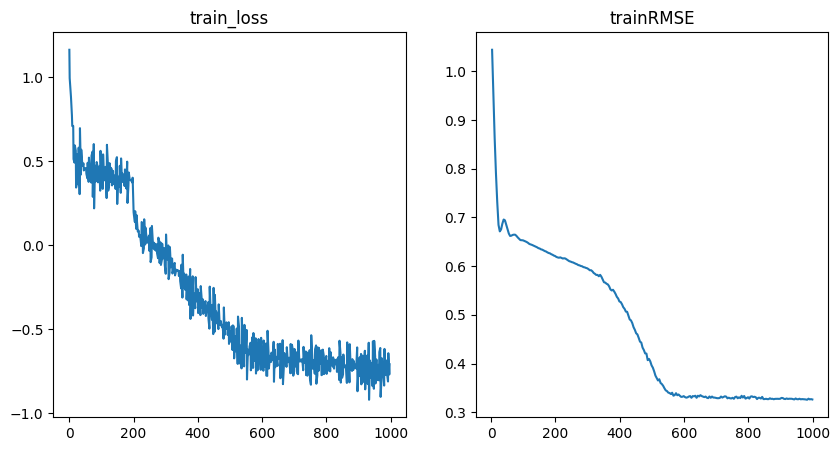
Training Metrics

To get some insights into how the training went of our underlying deterministic model, we can use the utility function to plot the training loss and RMSE metric.

fig = plot_training_metrics(
    os.path.join(my_temp_dir, "lightning_logs"), ["train_loss", "trainRMSE"]
)

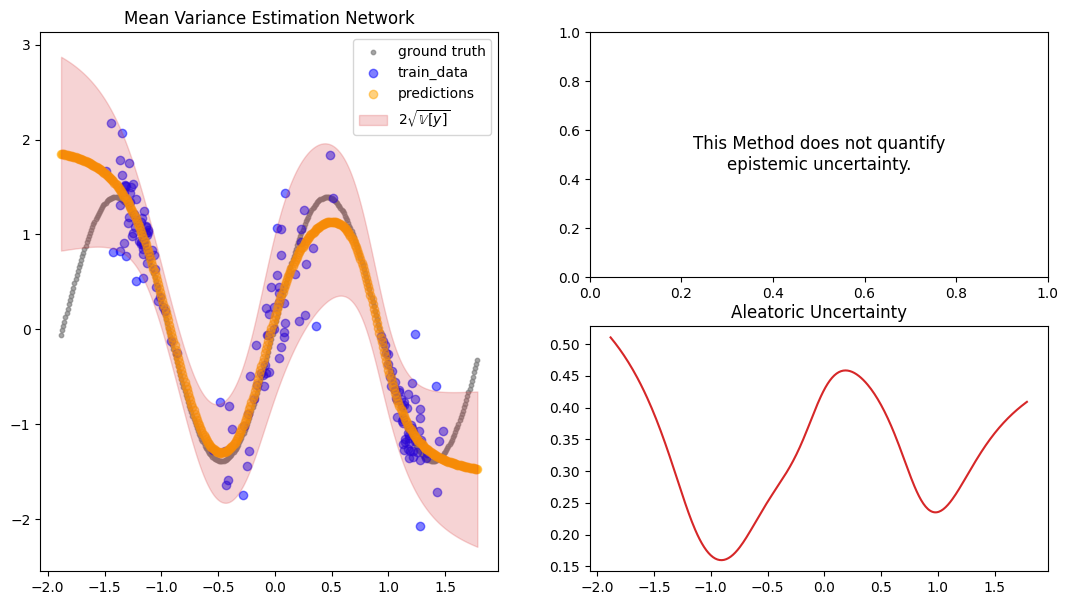
We can also make predictions with the underlying model.

deterministic_preds = deterministic_model.predict_step(
    X_gtext.to(deterministic_model.device)
)
fig = plot_predictions_regression(
    X_train,
    Y_train,
    X_gtext,
    Y_gtext,
    deterministic_preds["pred"].squeeze(-1),
    deterministic_preds["pred_uct"].squeeze(-1),
    aleatoric=deterministic_preds["aleatoric_uct"].squeeze(-1),
    title="Mean Variance Estimation Network",
)

Apply SWAG

We now have a deterministic model that can make predictions, however, we do not have any uncertainty around the network weights. SWAG is a Bayesian Approximation method to capture this uncertainty, and we will now apply it to obtain epistemic uncertainty.

swag_model = SWAGRegression(
    deterministic_model.model,
    max_swag_snapshots=30,
    snapshot_freq=1,
    num_mc_samples=50,
    swag_lr=1e-3,
    loss_fn=NLL(),
)
swag_trainer = Trainer(
    accelerator="cpu",
    max_epochs=20,  # number of epochs to fit swag
    log_every_n_steps=1,
    enable_progress_bar=False,
)

GPU available: False, used: False
TPU available: False, using: 0 TPU cores
/home/docs/checkouts/readthedocs.org/user_builds/lightning-uq-box/envs/latest/lib/python3.12/site-packages/lightning/pytorch/trainer/connectors/logger_connector/logger_connector.py:76: Starting from v1.9.0, `tensorboardX` has been removed as a dependency of the `lightning.pytorch` package, due to potential conflicts with other packages in the ML ecosystem. For this reason, `logger=True` will use `CSVLogger` as the default logger, unless the `tensorboard` or `tensorboardX` packages are found. Please `pip install lightning[extra]` or one of them to enable TensorBoard support by default
💡 Tip: For seamless cloud logging and experiment tracking, try installing [litlogger](https://pypi.org/project/litlogger/) to enable LitLogger, which logs metrics and artifacts automatically to the Lightning Experiments platform.

Prediction

For prediction we can either rely on the trainer.test() method or manually conduct a predict_step(). Using the trainer will save the predictions and some metrics to a CSV file, while the manual predict_step() with a single input tensor will generate a dictionary that holds the mean prediction as well as some other quantities of interest, for example the predicted standard deviation or quantile. The SWAG wrapper module will conduct the SWAG fitting procedure automatically before making the first prediction and will use it for any subsequent call to sample network weights for the desired number of Monte Carlo samples.

swag_trainer.fit(swag_model, datamodule=dm)

💡 Tip: For seamless cloud uploads and versioning, try installing [litmodels](https://pypi.org/project/litmodels/) to enable LitModelCheckpoint, which syncs automatically with the Lightning model registry.

  | Name         | Type             | Params | Mode  | FLOPs
------------------------------------------------------------------
0 | model        | MLP              | 5.3 K  | train | 0
1 | loss_fn      | NLL              | 0      | train | 0
2 | test_metrics | MetricCollection | 0      | train | 0
------------------------------------------------------------------
5.3 K     Trainable params
0         Non-trainable params
5.3 K     Total params
0.021     Total estimated model params size (MB)
15        Modules in train mode
0         Modules in eval mode
0         Total Flops
`Trainer.fit` stopped: `max_epochs=20` reached.

Evaluate Predictions

The constructed Data Module contains two possible test variable. X_test are IID samples from the same noise distribution as the training data, while X_gtext (“X ground truth extended”) are dense inputs from the underlying “ground truth” function without any noise that also extends the input range to either side, so we can visualize the method’s UQ tendencies when extrapolating beyond the training data range. Thus, we will use X_gtext for visualization purposes, but use X_test to compute uncertainty and calibration metrics because we want to analyse how well the method has learned the noisy data distribution.

preds = swag_model.predict_step(X_gtext.to(swag_model.device))

fig = plot_predictions_regression(
    X_train,
    Y_train,
    X_gtext,
    Y_gtext,
    preds["pred"],
    preds["pred_uct"],
    epistemic=preds["epistemic_uct"],
    aleatoric=preds["aleatoric_uct"],
    title="SWAG",
    show_bands=False,
)

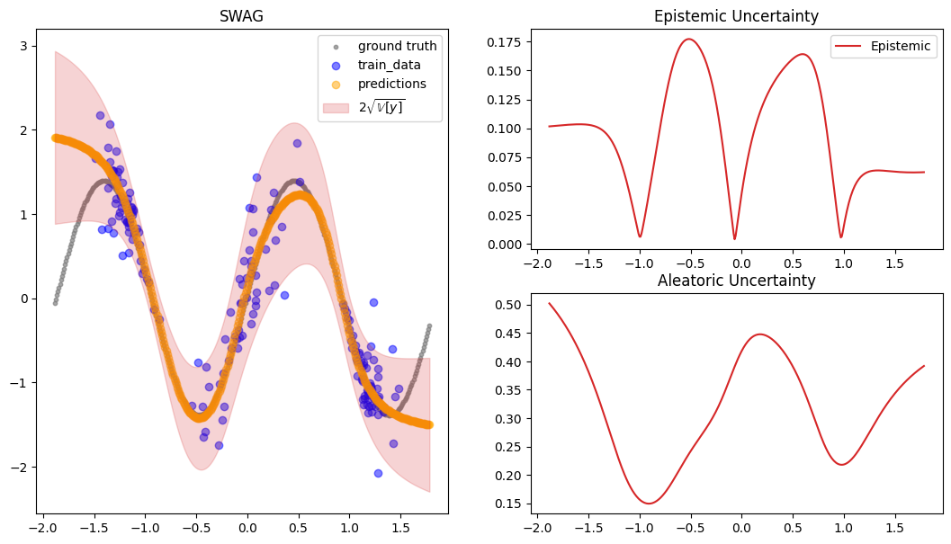
In the above plot we can observe, that we also now nave an estimate of the epistemic uncertainy with the SWAG method.

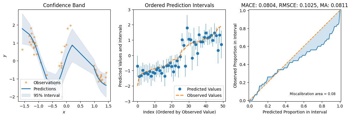
For some additional metrics relevant to UQ, we can use the great uncertainty-toolbox that gives us some insight into the calibration of our prediction.

preds = swag_model.predict_step(X_test.to(swag_model.device))

fig = plot_calibration_uq_toolbox(
    preds["pred"].cpu().numpy(),
    preds["pred_uct"].cpu().numpy(),
    Y_test.cpu().numpy(),
    X_test.cpu().numpy(),
)