ZigZag Classification MNIST#
In this notebook we will recreate the results of the MNIST notebook shown in the official repo. In particular, the evaluation scheme and code is the same as their notebook.
ZigZag was proposed by Durasov et al 2024.
Imports#
[1]:
import os
import tempfile
from functools import partial

import matplotlib.pyplot as plt
import numpy as np
import sklearn.metrics
import torch
import torch.nn as nn
import torch.nn.functional as F
import torchvision
from lightning import LightningDataModule, Trainer
from lightning.pytorch import seed_everything
from lightning.pytorch.loggers import CSVLogger

from lightning_uq_box.uq_methods import ZigZagClassification
from lightning_uq_box.viz_utils import plot_training_metrics

plt.rcParams["figure.figsize"] = [14, 5]

%load_ext autoreload
%autoreload 2
[2]:
seed_everything(0)
Seed set to 0
[2]:
0
[3]:
my_temp_dir = tempfile.mkdtemp()
Datamodule#
The following creates a quick Datamodule for the MNIST and MNIST Fashion Dataset so that we can easily train and evaluate our model. The MNIST Fashion dataset can be used as OOD evaluation.
[4]:
def collate_fn(batch):
    """Colate function for dataloader as dictionary."""
    images, targets = zip(*batch)
    images = torch.stack(images)
    targets = torch.tensor(targets)
    return {"input": images, "target": targets}


class MNISTDatamodule(LightningDataModule):
    def __init__(self, root: str, batch_size: int = 64, num_workers=0):
        super().__init__()
        self.batch_size = batch_size
        self.num_workers = num_workers
        self.root = root

    def setup(self, stage: str) -> None:
        """Setup data loader."""
        if stage in ["fit", "validate"]:
            mnist_train = torchvision.datasets.MNIST(
                self.root,
                train=True,
                download=True,
                transform=torchvision.transforms.Compose(
                    [
                        torchvision.transforms.ToTensor(),
                        torchvision.transforms.Normalize((0.1307,), (0.3081,)),
                    ]
                ),
            )
            self.mnist_train, self.mnist_val = torch.utils.data.random_split(
                mnist_train, [55000, 5000]
            )

        if stage in ["test"]:
            self.mnist_test = torchvision.datasets.MNIST(
                self.root,
                train=False,
                download=True,
                transform=torchvision.transforms.Compose(
                    [
                        torchvision.transforms.ToTensor(),
                        torchvision.transforms.Normalize((0.1307,), (0.3081,)),
                    ]
                ),
            )

    def train_dataloader(self):
        return torch.utils.data.DataLoader(
            self.mnist_train,
            batch_size=self.batch_size,
            num_workers=self.num_workers,
            collate_fn=collate_fn,
        )

    def val_dataloader(self):
        return torch.utils.data.DataLoader(
            self.mnist_val,
            batch_size=self.batch_size * 10,
            num_workers=self.num_workers,
            collate_fn=collate_fn,
        )

    def test_dataloader(self):
        return torch.utils.data.DataLoader(
            self.mnist_test,
            batch_size=self.batch_size * 10,
            num_workers=self.num_workers,
            collate_fn=collate_fn,
        )


class MNISTFashionDatamodule(MNISTDatamodule):
    """MNIST Fashion Datamodule"""

    def setup(self, stage: str) -> None:
        """Setup data loader."""
        if stage in ["fit", "validate"]:
            mnist_train = torchvision.datasets.FashionMNIST(
                self.root,
                train=True,
                download=True,
                transform=torchvision.transforms.Compose(
                    [
                        torchvision.transforms.ToTensor(),
                        torchvision.transforms.Normalize((0.1307,), (0.3081,)),
                    ]
                ),
            )
            self.mnist_train, self.mnist_val = torch.utils.data.random_split(
                mnist_train, [55000, 5000]
            )

        if stage in ["test"]:
            self.mnist_test = torchvision.datasets.FashionMNIST(
                self.root,
                train=False,
                download=True,
                transform=torchvision.transforms.Compose(
                    [
                        torchvision.transforms.ToTensor(),
                        torchvision.transforms.Normalize((0.1307,), (0.3081,)),
                    ]
                ),
            )
[5]:
datamodule = MNISTDatamodule(root="./data", batch_size=64, num_workers=2)
datamodule.setup("fit")
datamodule.setup("test")

fashion_dm = MNISTFashionDatamodule(root="./data", batch_size=64, num_workers=2)
fashion_dm.setup("test")
Example Training Samples#
[6]:
train_loader = datamodule.train_dataloader()
batch = next(iter(train_loader))
images, targets = batch["input"], batch["target"]

# Number of images you want to display
num_images = 10

# Create a figure and a row of subplots
fig, axes = plt.subplots(1, num_images, figsize=(15, 3))

# Plot each image on a separate subplot
for i in range(num_images):
    axes[i].imshow(images[i, 0], cmap="gray")
    axes[i].axis("off")  # Hide axis

plt.show()

Model and Training#
We use the same architecture they use in the notebook.
[7]:
class Net(nn.Module):
    def __init__(self):
        super().__init__()
        self.conv1 = nn.Conv2d(
            2, 10, kernel_size=5
        )  # modified first layer, takes 2-channel image as input
        self.conv2 = nn.Conv2d(10, 20, kernel_size=5)
        self.fc1 = nn.Linear(320, 50)
        self.fc2 = nn.Linear(50, 50)
        self.fc3 = nn.Linear(50, 10)
        self.activation = nn.LeakyReLU(negative_slope=0.01)

    def forward(self, x):
        x = self.activation(F.max_pool2d(self.conv1(x), 2))
        x = self.activation(F.max_pool2d(self.conv2(x), 2))
        x = x.view(-1, 320)
        x = self.activation(self.fc1(x))
        x = self.activation(self.fc2(x))
        x = self.fc3(x)
        return x
[8]:
zig_zag = ZigZagClassification(
    model=Net(),
    optimizer=partial(torch.optim.Adam, lr=1e-3),
    loss_fn=nn.CrossEntropyLoss(),
    blank_const=-20,
)
[9]:
logger = CSVLogger(my_temp_dir)
trainer = Trainer(
    max_epochs=5,
    accelerator="cpu",
    logger=logger,  # log training metrics for later evaluation
    enable_progress_bar=True,
    default_root_dir=my_temp_dir,
)
GPU available: False, used: False
TPU available: False, using: 0 TPU cores
IPU available: False, using: 0 IPUs
HPU available: False, using: 0 HPUs
[10]:
trainer.fit(zig_zag, datamodule)
Missing logger folder: /tmp/tmpg7ninxq5/lightning_logs

  | Name          | Type             | Params
---------------------------------------------------
0 | model         | Net              | 24.6 K
1 | loss_fn       | CrossEntropyLoss | 0
2 | train_metrics | MetricCollection | 0
3 | val_metrics   | MetricCollection | 0
4 | test_metrics  | MetricCollection | 0
---------------------------------------------------
24.6 K    Trainable params
0         Non-trainable params
24.6 K    Total params
0.099     Total estimated model params size (MB)
`Trainer.fit` stopped: `max_epochs=5` reached.
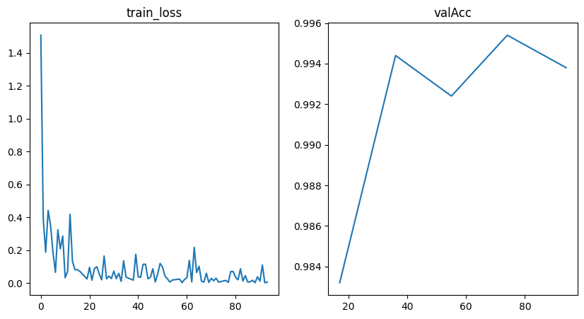
Training Metrics#
[11]:
fig = plot_training_metrics(
    os.path.join(my_temp_dir, "lightning_logs"), ["train_loss", "valAcc"]
)
Prediction Evaluation#
We evaluate predictions across in distribution and out of distribution samples, for the latter with the MNISTFashion Dataset. We use the same code as their notebook.
[12]:
def process_data(dataloader, is_in_distribution=True):
    uncertainties = np.array([])
    labels = np.array([])
    target = np.array([])
    pred = np.array([])
    target_acc = np.array([])
    images_to_viz = []

    for batch in dataloader:
        images, targs = batch["input"], batch["target"]
        preds = zig_zag.predict_step(images)
        uncertainties = np.concatenate([uncertainties, preds["pred_uct"]])
        labels = np.concatenate(
            [labels, np.zeros_like(preds["pred_uct"])]
            if is_in_distribution
            else [labels, np.ones_like(preds["pred_uct"])]
        )
        target_acc = np.concatenate(
            [target_acc, (preds["pred"].argmax(1) == targs).numpy()]
        )
        target = np.concatenate([target, targs.numpy()])
        pred = np.concatenate([pred, preds["pred"].argmax(1)])
        images_to_viz.append(images)

    images_to_viz = torch.cat(images_to_viz).numpy()
    return uncertainties, labels, target, pred, target_acc, images_to_viz


# Process IN and OUT distribution data
uncertainties_in, labels_in, target_in, pred_in, target_acc_in, images_to_viz_in = (
    process_data(datamodule.test_dataloader(), is_in_distribution=True)
)
(
    uncertainties_out,
    labels_out,
    target_out,
    pred_out,
    target_acc_out,
    images_to_viz_out,
) = process_data(fashion_dm.test_dataloader(), is_in_distribution=False)

# Concatenate IN and OUT for combined evaluation
uncertainties_combined = np.concatenate([uncertainties_in, uncertainties_out])
labels_combined = np.concatenate([labels_in, labels_out])
target_acc_combined = np.concatenate([target_acc_in, target_acc_out])
target_combined = np.concatenate([target_in, target_out])
images_to_viz_combined = np.concatenate([images_to_viz_in, images_to_viz_out])
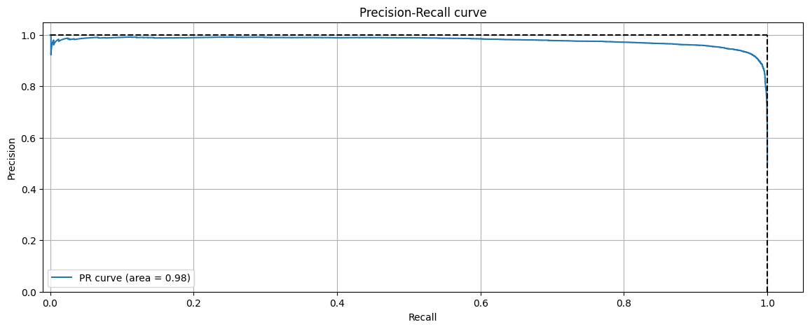
[13]:
roc_auc = sklearn.metrics.roc_auc_score(labels_combined, uncertainties_combined)
precision, recall, thresholds = sklearn.metrics.precision_recall_curve(
    labels_combined, uncertainties_combined
)
pr_auc = sklearn.metrics.auc(recall, precision)

# evaluate ROC- and PR-AUC metrics, see https://arxiv.org/abs/1802.10501 for more details
print(f"ROC AUC: {roc_auc:.4f} ")
print(f"PR AUC: {pr_auc:.4f}")

# Plot ROC curve
fpr, tpr, _ = sklearn.metrics.roc_curve(labels_combined, uncertainties_combined)
plt.figure()
plt.plot(fpr, tpr, label=f"ROC curve (area = {roc_auc:.2f})")
plt.plot([0, 1], [0, 1], "g--", label="Random classifier")
plt.hlines(1, xmin=0, xmax=1, color="k", linestyle="--")
plt.vlines(0, ymin=0, ymax=1, color="k", linestyle="--")
plt.xlim([-0.01, 1.05])
plt.ylim([0.0, 1.05])
plt.xlabel("False Positive Rate")
plt.ylabel("True Positive Rate")
plt.title("Receiver Operating Characteristic")
plt.grid()
plt.legend(loc="lower right")
plt.show()

# Plot PR curve
plt.figure()
plt.plot(recall, precision, label=f"PR curve (area = {pr_auc:.2f})")
plt.hlines(1, xmin=0, xmax=1, color="k", linestyle="--")
plt.vlines(1, ymin=0, ymax=1, color="k", linestyle="--")
plt.xlabel("Recall")
plt.ylabel("Precision")
plt.title("Precision-Recall curve")
plt.xlim([-0.01, 1.05])
plt.ylim([0.0, 1.05])
plt.grid()
plt.legend(loc="lower left")
plt.show()
ROC AUC: 0.9849
PR AUC: 0.9792

Some Visual Examples#
[14]:
def visualize_samples(uncertainties, preds, targets, images_to_viz):
    # Sort the samples by uncertainty
    sorted_indices = sorted(range(len(uncertainties)), key=lambda i: uncertainties[i])
    sorted_images = [images_to_viz[i] for i in sorted_indices]
    sorted_uncertainties = [uncertainties[i] for i in sorted_indices]
    sorted_preds = [preds[i] for i in sorted_indices]
    sorted_targets = [targets[i] for i in sorted_indices]

    # Select the three highest and three lowest uncertainty samples
    selected_images = sorted_images[:3] + sorted_images[-3:]
    selected_uncertainties = sorted_uncertainties[:3] + sorted_uncertainties[-3:]
    selected_preds = sorted_preds[:3] + sorted_preds[-3:]
    selected_targets = sorted_targets[:3] + sorted_targets[-3:]

    plt.figure(figsize=(15, 5))
    for i in range(6):
        plt.subplot(2, 3, i + 1)
        plt.imshow(selected_images[i].squeeze(), cmap="gray")
        plt.title(
            f"Pred: {selected_preds[i]}, Target: {selected_targets[i]}, Uncertainty: {selected_uncertainties[i]:.2f}"
        )
        plt.axis("off")
    plt.tight_layout()
    plt.show()
In Distribution#
[15]:
visualize_samples(uncertainties_in, pred_in, target_in, images_to_viz_in)

Out of Distribution#
[16]:
visualize_samples(uncertainties_out, pred_out, target_out, images_to_viz_out)

Uncertainty Calibration Evaluation#
For calibration evaluation, we also use their evaluation scheme, more specifically the rAULC metric. For more details, see https://arxiv.org/pdf/2107.00649.
[17]:
uncertainties = np.array([])
targets = np.array([])
target_acc = np.array([])
images_to_viz = []

# IN Distribution
for batch in datamodule.test_dataloader():
    images, targs = batch["input"], batch["target"]
    preds = zig_zag.predict_step(images)
    uncertainties = np.concatenate([uncertainties, preds["pred_uct"]])
    targets = np.concatenate([targets, targs])
    target_acc = np.concatenate(
        [target_acc, (preds["pred"].argmax(1) == targs).numpy()]
    )
    images_to_viz.append(images)

images_to_viz = np.concatenate(images_to_viz)
[18]:
def AULC(accs, uncertainties):
    idxs = np.argsort(uncertainties)
    error_s = accs[idxs]

    mean_error = error_s.mean()
    error_csum = np.cumsum(error_s)

    Fs = error_csum / np.arange(1, len(error_s) + 1)
    s = 1 / len(Fs)
    return -1 + s * Fs.sum() / mean_error, Fs


def rAULC(uncertainties, accs):
    perf_aulc, Fsp = AULC(accs, -accs.astype("float"))
    curr_aulc, Fsc = AULC(accs, uncertainties)
    print(perf_aulc, curr_aulc)
    return curr_aulc / perf_aulc, Fsp, Fsc


res, r1, r2 = rAULC(uncertainties, target_acc)
print(res)

plt.plot(range(len(r1)), r1)
plt.plot(range(len(r1)), r2)
plt.grid()
0.021222563964778285 0.02053685294952734
0.9676895300497633
