Bayesian Neural Networks with Latent Variables#
Theoretic Foundation#
BNN with latent variables (LVs) extend BNNs with VI to encompass LVs that model aleatoric uncertainty. The BNN+LV model is proposed in Depeweg, 2018.
The likelihood is given by
The prior on the weights is obtained as for BNNs with VI and is given by,
where \(w_{hj, l}\) is the h-th row and the j-th column of weight matrix \(\theta_L\) at layer index \(L\) and \(\lambda\) is the prior variance. Note that as we use partially stochastic networks, the above may contain less factors \(\mathcal{N}(w_{hj, l} \vert 0, \lambda)\) depending on how many layers are stochastic. The prior distribution of the latent variables z is given by
where \(\gamma\) is the prior variance.
Then, with the assumed likelihood function and prior, a posterior over the weights \(\theta\) and latent variables \(z\) is obtained via Bayes’ rule:
The approximate the posterior is given by
Now the parameters \(m^w_{hj,l}\),\(v^w_{hj,l}\) and \(m^z_i\), \(v^z_i\) can be obtained by minimizing a divergence between \(p(\theta, z| \mathcal{D})\). Here the following approximation of the \(\alpha\) divergence, as proposed in Lobato, 2016 and Depeweg, 2016, is used,
where \(Z_n\) is the normalising constant of the exponential form of approximate the posterior and \(f(\Theta)\) and \(f_n(z_n)\) are functions depending on the parameters of the distributions of the prior on the weights and of the prior distribution of the latent variables, see Depeweg, 2016 for details. In order to make this optimization problem scalable, SGD with mini-batches is used, and the expectation over \(q\) is approximated with an average over \(K\) samples drawn from \(q\).
The posterior predictive distribution is given by,
The network prediction \(f_{\theta}(x_{\star}, z_{\star})\) uses \(z_{\star}\) sampled from the prior distribution \(\mathcal{N}(z_{\star} \vert 0, \gamma)\) because this is the only evidence we have about the latent variable for a new data point since all data points are assumed to be independent. However, the above posterior predictive distribution is intractable in this form. So instead we use sampling from the posterior distribution of the weights. The mean prediction is then given by the mean prediction of samples and the predictive uncertainty is obtained as standard deviation of samples from the approximation to the posterior predictive distribution.
[1]:
%%capture
%pip install git+https://github.com/lightning-uq-box/lightning-uq-box.git
Imports#
[2]:
import os
import tempfile
from functools import partial

import matplotlib.pyplot as plt
import torch
import torch.nn as nn
from lightning import Trainer
from lightning.pytorch import seed_everything
from lightning.pytorch.loggers import CSVLogger

from lightning_uq_box.datamodules import ToyHeteroscedasticDatamodule
from lightning_uq_box.models import MLP
from lightning_uq_box.uq_methods import BNN_LV_VI_Batched_Regression
from lightning_uq_box.viz_utils import (
    plot_calibration_uq_toolbox,
    plot_predictions_regression,
    plot_toy_regression_data,
    plot_training_metrics,
)

plt.rcParams["figure.figsize"] = [14, 5]
INFO:root:Asdfghjkl backend not available since the old asdfghjkl dependency is not installed. If you want to use it, run: pip install git+https://git@github.com/wiseodd/asdl@asdfghjkl
[3]:
seed_everything(0) # seed everything for reproducibility
Seed set to 0
[3]:
0
We define a temporary directory to look at some training metrics and results.
[4]:
my_temp_dir = tempfile.mkdtemp()
Datamodule#
To demonstrate the method, we will make use of a Toy Regression Example that is defined as a Lightning Datamodule. While this might seem like overkill for a small toy problem, we think it is more helpful how the individual pieces of the library fit together so you can train models on more complex tasks.
[5]:
dm = ToyHeteroscedasticDatamodule(batch_size=50, n_points=800)

X_train, Y_train, train_loader, X_test, Y_test, test_loader, X_gtext, Y_gtext = (
    dm.X_train,
    dm.Y_train,
    dm.train_dataloader(),
    dm.X_test,
    dm.Y_test,
    dm.test_dataloader(),
    dm.X_gtext,
    dm.Y_gtext,
)
[6]:
fig = plot_toy_regression_data(X_train, Y_train, X_test, Y_test)

Model#
For our Toy Regression problem, we will use a simple Multi-layer Perceptron (MLP) that will be converted to a BNN as well as a Latent Variable Network.
[7]:
bnn = MLP(n_inputs=1, n_hidden=[50, 50, 50], n_outputs=1, activation_fn=nn.ReLU())
latent_net = MLP(
    n_inputs=2,  # num_input_features + num_target_dim
    n_outputs=2,  # 2 * lv_latent_dim
    n_hidden=[20],
    activation_fn=nn.ReLU(),
)
bnn, latent_net
[7]:
(MLP(
   (model): Sequential(
     (0): Linear(in_features=1, out_features=50, bias=True)
     (1): ReLU()
     (2): Dropout(p=0.0, inplace=False)
     (3): Linear(in_features=50, out_features=50, bias=True)
     (4): ReLU()
     (5): Dropout(p=0.0, inplace=False)
     (6): Linear(in_features=50, out_features=50, bias=True)
     (7): ReLU()
     (8): Dropout(p=0.0, inplace=False)
     (9): Linear(in_features=50, out_features=1, bias=True)
   )
 ),
 MLP(
   (model): Sequential(
     (0): Linear(in_features=2, out_features=20, bias=True)
     (1): ReLU()
     (2): Dropout(p=0.0, inplace=False)
     (3): Linear(in_features=20, out_features=2, bias=True)
   )
 ))
With an underlying neural network, we can now use our desired UQ-Method as a sort of wrapper. All UQ-Methods are implemented as LightningModule that allow us to concisely organize the code and remove as much boilerplate code as possible.
The BNN_LV_VI_Batched_Regression model enables us to chose the layers of our network we want to make stochastic via the stochastic_module_names argument. This can be done by either a list of module names or a list of module numbers. For example, stochastic_module_name = [-1] would only make the last layer stochastic while all other layers remain determinstic. The default value of None makes all layers stochastic. The hyperparameter alpha determines how the Gaussian approximation of the
posterior fits the posterior of the weights, see Figure 1, Depeweg, 2016.
[8]:
bnn_vi_model = BNN_LV_VI_Batched_Regression(
    bnn,
    latent_net,
    optimizer=partial(torch.optim.Adam, lr=1e-3),
    num_training_points=X_train.shape[0],
    n_mc_samples_train=10,
    n_mc_samples_test=50,
    output_noise_scale=1.3,
    prior_mu=0.0,
    prior_sigma=1.0,
    posterior_mu_init=0.0,
    posterior_rho_init=-6.0,
    alpha=1e-03,
    bayesian_layer_type="reparameterization",
)
Trainer#
Now that we have a LightningDataModule and a UQ-Method as a LightningModule, we can conduct training with a Lightning Trainer. It has tons of options to make your life easier, so we encourage you to check the documentation.
[9]:
logger = CSVLogger(my_temp_dir)
trainer = Trainer(
    max_epochs=250,  # number of epochs we want to train
    logger=logger,  # log training metrics for later evaluation
    log_every_n_steps=1,
    enable_checkpointing=False,
    enable_progress_bar=False,
    limit_val_batches=0.0,  # skip validation runs
    default_root_dir=my_temp_dir,
)
GPU available: False, used: False
TPU available: False, using: 0 TPU cores
HPU available: False, using: 0 HPUs
Training our model is now easy:
[10]:
trainer.fit(bnn_vi_model, dm)
  | Name            | Type                  | Params | Mode
------------------------------------------------------------------
0 | model           | MLP                   | 10.5 K | train
1 | train_metrics   | MetricCollection      | 0      | train
2 | val_metrics     | MetricCollection      | 0      | train
3 | test_metrics    | MetricCollection      | 0      | train
4 | prediction_head | LinearVariational     | 102    | train
5 | lv_net          | LatentVariableNetwork | 102    | train
  | other params    | n/a                   | 1      | n/a
------------------------------------------------------------------
10.7 K    Trainable params
0         Non-trainable params
10.7 K    Total params
0.043     Total estimated model params size (MB)
30        Modules in train mode
0         Modules in eval mode
`Trainer.fit` stopped: `max_epochs=250` reached.
Training Metrics#
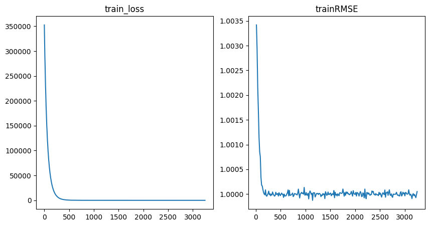
To get some insights into how the training went, we can use the utility function to plot the training loss and RMSE metric.
[11]:
fig = plot_training_metrics(
    os.path.join(my_temp_dir, "lightning_logs"), ["train_loss", "trainRMSE"]
)
Prediction#
[12]:
# save predictions
trainer.test(bnn_vi_model, dm)
────────────────────────────────────────────────────────────────────────────────────────────────────────────────────────
       Test metric             DataLoader 0
────────────────────────────────────────────────────────────────────────────────────────────────────────────────────────
         testMAE            0.8813395500183105
         testR2            -0.01376199722290039
        testRMSE            0.9811044931411743
────────────────────────────────────────────────────────────────────────────────────────────────────────────────────────
[12]:
[{'testMAE': 0.8813395500183105,
  'testR2': -0.01376199722290039,
  'testRMSE': 0.9811044931411743}]
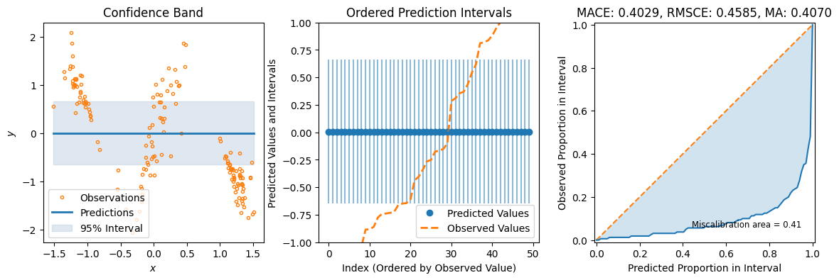
Evaluate Predictions#
The constructed Data Module contains two possible test variable. X_test are IID samples from the same noise distribution as the training data, while X_gtext (“X ground truth extended”) are dense inputs from the underlying “ground truth” function without any noise that also extends the input range to either side, so we can visualize the method’s UQ tendencies when extrapolating beyond the training data range. Thus, we will use X_gtext for visualization purposes, but use X_test to
compute uncertainty and calibration metrics because we want to analyse how well the method has learned the noisy data distribution.
[13]:
preds = bnn_vi_model.predict_step(X_gtext)

fig = plot_predictions_regression(
    X_train,
    Y_train,
    X_gtext,
    Y_gtext,
    preds["pred"],
    preds["pred_uct"],
    epistemic=preds["epistemic_uct"],
    aleatoric=preds["aleatoric_uct"],
    title="title here",
)
INFO:matplotlib.mathtext:Substituting symbol V from STIXNonUnicode
INFO:matplotlib.mathtext:Substituting symbol V from STIXNonUnicode

For some additional metrics relevant to UQ, we can use the great uncertainty-toolbox that gives us some insight into the calibration of our prediction.
[14]:
preds = bnn_vi_model.predict_step(X_test)
fig = plot_calibration_uq_toolbox(
    preds["pred"].numpy(),
    preds["pred_uct"].numpy(),
    Y_test.cpu().numpy(),
    X_test.cpu().numpy(),
)
Additional Resources#
Links to othere related literature that might be interesting.