Laplace Approximation#
[1]:
%%capture
%pip install git+https://github.com/lightning-uq-box/lightning-uq-box.git
Theoretic Foundation#
The Laplace Approximation was originally introduced by MacKay, 1992. Then, the Laplace Approximation has been adapted to modern neural networks by Ritter, 2018 and Daxberger, 2021 and is an approximate Bayesian method. The goal of the Laplace Approximation is to use a second-order Taylor expansion around the fitted MAP estimate and yield a posterior approximation over the model parameters via a full-rank, diagonal or Kronecker-factorized approach. In order for the Laplace Approximation to be computationally feasible for larger network architectures, we use the Laplace library to include approaches, such as subnetwork selection that have been for example proposed by Daxberger, 2021.
The general idea of the Laplace Approximation to obtain a distribution over the network parameters is to approximate the posterior with a Gaussian distribution centered at the MAP estimate of the parameters Daxberger, 2021. In this setting, we define a prior distribution \(p(\theta)\) over our network parameters. Because modern neural networks consists of millions of parameters, obtaining a posterior distribution over the weights \(\theta\) is intractable. The LA takes MAP estimate of the parameters \(\theta_{MAP}\) from a trained network \(f_{\theta_{MAP}}(x) = \mu_{\theta_{MAP}}(x)\) and constructs a Gaussian distribution around it. The parameters \(\theta_{MAP}\) are obtained by
where \(\mathcal{L}\) is the mean squared error or also referred to as the \(\ell^2\) loss, \(\mathcal{L}(\theta; \mathcal{D}) := -\sum_{i=1}^n log(p(y_i|f_{\theta}(x_i)))\) and we chose the posterior \(p(y_i|f_{\theta}(x_i))\) to be a Gaussian with constant variance \(\sigma^2\), such that the loss is the mean squared error and a homoskedastic noise model is assumed. Then with Bayes Theorem, as in Daxberger, 2021, one can relate the posterior to the loss,
with \(Z = \int p(D\vert\theta)p(\theta) d\theta\). Now a second-order expansion of \(\mathcal{L}\) around \(\theta_{MAP}\) is used to construct a Gaussian approximation to the posterior \(p(\theta|D)\):
The term with the first order derivative is zero as the loss is evaluated at a minimum \(\theta_{MAP}\) Murphy, 2022, and, further, one assumes that the first term is neglible as the loss is evaluated at \(\theta = \theta_{MAP}\). Then taking the expontential of both sides allows to identify, after normalization, the Laplace approximation,
\begin{align*} p(\theta|D) \approx \mathcal{N}(\theta_{MAP}, \Sigma) && \text{with} \qquad \Sigma = (\nabla_{\theta}^2 \mathcal{L}(\theta; D)\vert \theta_{MAP})^{-1}. \end{align*}
As the covariance is just the inverse Hessian of the loss, with \(\theta_{MAP}\in \mathcal{R}^W\) and \(H^{-1}\in \mathcal{R}^{W\times W}\), with \(W\) being the number of weights, we get the posterior distribution
The computation of the Hessian term is still expensive. Therefore, further approximations are introduced in practice, most commonly the Generalized Gauss-Newton matrix \cite{martens2020new}. This takes the following form:
where \(J_n\in \mathcal{R}^{O\times W}\) is the Jacobian of the model outputs with respect to the parameters \(\theta\) and \(H_n\in\mathcal{R}^{O\times O}\) is the Hessian of the negative log-likelihood with respect to the model outputs, where \(O\) denotes the model output size and \(W\) the number of parameters.
During prediction we cannot compute the full posterior predictive distribution but instead resort to approximations. One strategy is to do sampling \(\theta_s \sim p(\theta|D)\) for \(s \in \{1, ...,S\}\) to approximate the predictions, however, Immer et al. 2021 suggested that a linearization of the form \(f_{\theta}(x)=f_{\theta_{MAP}}(x)+ J_{\theta_{MAP}}(\theta-\theta_{MAP})\) works better in practice and this is also the default in the Laplace library.
and obtain the predictive uncertainty by
The implementation is a wrapper around a model from the fantastic Laplace library so all the available options for subnet strategies can be found in their docs.
Imports#
[2]:
import os
import tempfile
from functools import partial

import matplotlib.pyplot as plt
import torch
import torch.nn as nn
from laplace import Laplace
from lightning import Trainer
from lightning.pytorch import seed_everything
from lightning.pytorch.loggers import CSVLogger

from lightning_uq_box.datamodules import ToyHeteroscedasticDatamodule
from lightning_uq_box.models import MLP
from lightning_uq_box.uq_methods import DeterministicRegression, LaplaceRegression
from lightning_uq_box.viz_utils import (
    plot_calibration_uq_toolbox,
    plot_predictions_regression,
    plot_toy_regression_data,
    plot_training_metrics,
)

plt.rcParams["figure.figsize"] = [14, 5]
[3]:
seed_everything(0) # seed everything for reproducibility
INFO: Seed set to 0
INFO:lightning.fabric.utilities.seed:Seed set to 0
[3]:
0
We define a temporary directory to look at some training metrics and results.
[4]:
my_temp_dir = tempfile.mkdtemp()
Datamodule#
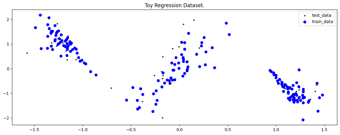
To demonstrate the method, we will make use of a Toy Regression Example that is defined as a Lightning Datamodule. While this might seem like overkill for a small toy problem, we think it is more helpful how the individual pieces of the library fit together so you can train models on more complex tasks.
[5]:
dm = ToyHeteroscedasticDatamodule()

X_train, Y_train, train_loader, X_test, Y_test, test_loader, X_gtext, Y_gtext = (
    dm.X_train,
    dm.Y_train,
    dm.train_dataloader(),
    dm.X_test,
    dm.Y_test,
    dm.test_dataloader(),
    dm.X_gtext,
    dm.Y_gtext,
)
[6]:
fig = plot_toy_regression_data(X_train, Y_train, X_test, Y_test)
Model#
For our Toy Regression problem, we will use a simple Multi-layer Perceptron (MLP) that you can configure to your needs. For the documentation of the MLP see here.
[7]:
network = MLP(n_inputs=1, n_hidden=[50, 50], n_outputs=1, activation_fn=nn.Tanh())
network
[7]:
MLP(
  (model): Sequential(
    (0): Linear(in_features=1, out_features=50, bias=True)
    (1): Tanh()
    (2): Dropout(p=0.0, inplace=False)
    (3): Linear(in_features=50, out_features=50, bias=True)
    (4): Tanh()
    (5): Dropout(p=0.0, inplace=False)
    (6): Linear(in_features=50, out_features=1, bias=True)
  )
)
For the Laplace model, we first train a plain deterministic model to obtain a MAP estimate of the weights via the standard MSE loss. Subsequently, we fit the Laplace Approximation to obtain an estimate of the epistemic uncertainty for predictions.
[8]:
deterministic_model = DeterministicRegression(
    model=network,
    optimizer=partial(torch.optim.Adam, lr=1e-2),
    loss_fn=torch.nn.MSELoss(),
)
Trainer#
Now that we have a LightningDataModule and base model, we can conduct training with a Lightning Trainer. It has tons of options to make your life easier, so we encourage you to check the documentation.
[9]:
logger = CSVLogger(my_temp_dir)
trainer = Trainer(
    max_epochs=100,  # number of epochs we want to train
    logger=logger,  # log training metrics for later evaluation
    log_every_n_steps=1,
    enable_checkpointing=False,
    enable_progress_bar=False,
)
INFO: GPU available: False, used: False
INFO:lightning.pytorch.utilities.rank_zero:GPU available: False, used: False
INFO: TPU available: False, using: 0 TPU cores
INFO:lightning.pytorch.utilities.rank_zero:TPU available: False, using: 0 TPU cores
INFO: HPU available: False, using: 0 HPUs
INFO:lightning.pytorch.utilities.rank_zero:HPU available: False, using: 0 HPUs
Training our model is now easy:
[10]:
trainer.fit(deterministic_model, dm)
INFO:
  | Name          | Type             | Params | Mode
-----------------------------------------------------------
0 | model         | MLP              | 2.7 K  | train
1 | loss_fn       | MSELoss          | 0      | train
2 | train_metrics | MetricCollection | 0      | train
3 | val_metrics   | MetricCollection | 0      | train
4 | test_metrics  | MetricCollection | 0      | train
-----------------------------------------------------------
2.7 K     Trainable params
0         Non-trainable params
2.7 K     Total params
0.011     Total estimated model params size (MB)
21        Modules in train mode
0         Modules in eval mode
INFO:lightning.pytorch.callbacks.model_summary:
  | Name          | Type             | Params | Mode
-----------------------------------------------------------
0 | model         | MLP              | 2.7 K  | train
1 | loss_fn       | MSELoss          | 0      | train
2 | train_metrics | MetricCollection | 0      | train
3 | val_metrics   | MetricCollection | 0      | train
4 | test_metrics  | MetricCollection | 0      | train
-----------------------------------------------------------
2.7 K     Trainable params
0         Non-trainable params
2.7 K     Total params
0.011     Total estimated model params size (MB)
21        Modules in train mode
0         Modules in eval mode
INFO: `Trainer.fit` stopped: `max_epochs=100` reached.
INFO:lightning.pytorch.utilities.rank_zero:`Trainer.fit` stopped: `max_epochs=100` reached.
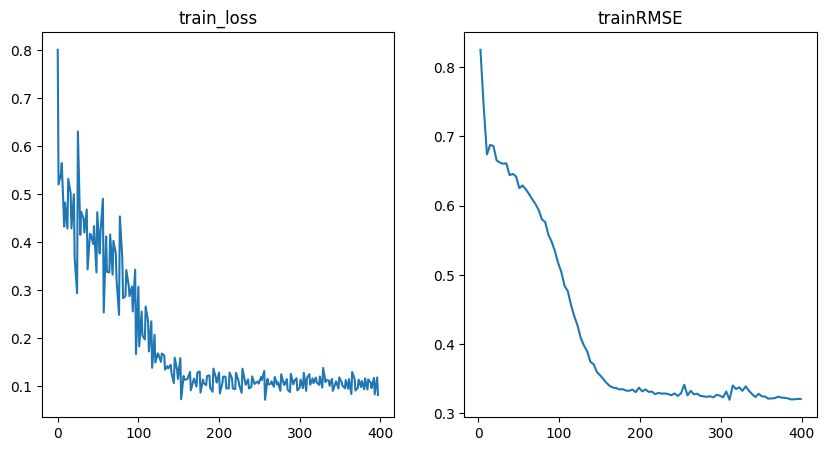
Training Metrics#
To get some insights into how the training went, we can use the utility function to plot the training loss and RMSE metric.
[11]:
fig = plot_training_metrics(
    os.path.join(my_temp_dir, "lightning_logs"), ["train_loss", "trainRMSE"]
)
Fit Laplace#
We will utilize the great Laplace Library that allows you to define different flavors of Laplace approximations. For small networks like in this example, one can fit the Laplace approximation over all weights, but this is not feasible for large million-parameter networks. In those cases, on can resort to a “last-layer” approximation, where only the last layer weights are stochastic, while all other weights are deterministic. This behavior is controlled
with the subset_of_weights parameter. This is chosen in combination with the structure of the Hessian that is fitted, see the hessian_structure parameter. Check their documentation for details. The Lightning-UQ-Box provides a wrapper so that the workflow is the same as with any other implemented UQ-Method.
One can also tune the prior precision and or sigma noise values after the Laplace fitting procedure with the argument tune_prior_precision=True and tune_sigma_noise=True otherwise, the prediction will rely on the default sigma_noise values passed to the Laplace class for an estimate of aleatoric uncertainty under a homoscedastic noise assumption. For a related discussion one can look at this GitHub issue.
[12]:
la = Laplace(
    deterministic_model.model,
    "regression",
    subset_of_weights="last_layer",
    hessian_structure="full",
    sigma_noise=0.4,
)


laplace_model = LaplaceRegression(laplace_model=la, tune_prior_precision=True)

trainer = Trainer(default_root_dir=my_temp_dir)
INFO: GPU available: False, used: False
INFO:lightning.pytorch.utilities.rank_zero:GPU available: False, used: False
INFO: TPU available: False, using: 0 TPU cores
INFO:lightning.pytorch.utilities.rank_zero:TPU available: False, using: 0 TPU cores
INFO: HPU available: False, using: 0 HPUs
INFO:lightning.pytorch.utilities.rank_zero:HPU available: False, using: 0 HPUs
/home/docs/checkouts/readthedocs.org/user_builds/lightning-uq-box/envs/stable/lib/python3.12/site-packages/lightning/pytorch/trainer/connectors/logger_connector/logger_connector.py:75: Starting from v1.9.0, `tensorboardX` has been removed as a dependency of the `lightning.pytorch` package, due to potential conflicts with other packages in the ML ecosystem. For this reason, `logger=True` will use `CSVLogger` as the default logger, unless the `tensorboard` or `tensorboardX` packages are found. Please `pip install lightning[extra]` or one of them to enable TensorBoard support by default
Prediction#
For prediction we can either rely on the trainer.test() method or manually conduct a predict_step(). Using the trainer will save the predictions and some metrics to a CSV file, while the manual predict_step() with a single input tensor will generate a dictionary that holds the mean prediction as well as some other quantities of interest, for example the predicted standard deviation or quantile. The Laplace wrapper module will conduct the Laplace fitting procedure automatically before
making the first prediction and will use it for any subsequent call. Originally, this was done through sampling and multiple forward passes, however, Immer et al. 2021 showed that a linearization of the model achieves better performance in practice: \(f_{\theta}(x)=f_{\theta_{MAP}}(x)+ J_{\theta_{MAP}}(\theta-\theta_{MAP})\) and that is the current default implementation. However, arguments can be passed to the class or the individual predict step to
choose between the following procedures of sampling as pred_type="glm" (linearization) or pred_type="nn" (sampling).
[13]:
trainer.test(laplace_model, dm)
  0%|          | 0/100 [00:00<?, ?it/s]
  0%|          | 0/100 [00:00<?, ?it/s, neg_marglik=76.09431457519531]
  0%|          | 0/100 [00:00<?, ?it/s, neg_marglik=76.09175872802734]
  0%|          | 0/100 [00:00<?, ?it/s, neg_marglik=76.08889770507812]
  0%|          | 0/100 [00:00<?, ?it/s, neg_marglik=76.08636474609375]
  0%|          | 0/100 [00:00<?, ?it/s, neg_marglik=76.08379364013672]
  0%|          | 0/100 [00:00<?, ?it/s, neg_marglik=76.08119201660156]
  0%|          | 0/100 [00:00<?, ?it/s, neg_marglik=76.07830047607422]
  0%|          | 0/100 [00:00<?, ?it/s, neg_marglik=76.07579803466797]
  0%|          | 0/100 [00:00<?, ?it/s, neg_marglik=76.07322692871094]
  0%|          | 0/100 [00:00<?, ?it/s, neg_marglik=76.07044982910156]
  0%|          | 0/100 [00:00<?, ?it/s, neg_marglik=76.06790161132812]
  0%|          | 0/100 [00:00<?, ?it/s, neg_marglik=76.06524658203125]
  0%|          | 0/100 [00:00<?, ?it/s, neg_marglik=76.06260681152344]
  0%|          | 0/100 [00:00<?, ?it/s, neg_marglik=76.0599365234375]
  0%|          | 0/100 [00:00<?, ?it/s, neg_marglik=76.05730438232422]
  0%|          | 0/100 [00:00<?, ?it/s, neg_marglik=76.05452728271484]
  0%|          | 0/100 [00:00<?, ?it/s, neg_marglik=76.05195617675781]
  0%|          | 0/100 [00:00<?, ?it/s, neg_marglik=76.04916381835938]
  0%|          | 0/100 [00:00<?, ?it/s, neg_marglik=76.04685974121094]
  0%|          | 0/100 [00:00<?, ?it/s, neg_marglik=76.0442123413086]
  0%|          | 0/100 [00:00<?, ?it/s, neg_marglik=76.04141235351562]
  0%|          | 0/100 [00:00<?, ?it/s, neg_marglik=76.03900146484375]
 22%|██▏       | 22/100 [00:00<00:00, 214.35it/s, neg_marglik=76.03900146484375]
 22%|██▏       | 22/100 [00:00<00:00, 214.35it/s, neg_marglik=76.03621673583984]
 22%|██▏       | 22/100 [00:00<00:00, 214.35it/s, neg_marglik=76.03351593017578]
 22%|██▏       | 22/100 [00:00<00:00, 214.35it/s, neg_marglik=76.03106689453125]
 22%|██▏       | 22/100 [00:00<00:00, 214.35it/s, neg_marglik=76.02828216552734]
 22%|██▏       | 22/100 [00:00<00:00, 214.35it/s, neg_marglik=76.02579498291016]
 22%|██▏       | 22/100 [00:00<00:00, 214.35it/s, neg_marglik=76.02302551269531]
 22%|██▏       | 22/100 [00:00<00:00, 214.35it/s, neg_marglik=76.02046203613281]
 22%|██▏       | 22/100 [00:00<00:00, 214.35it/s, neg_marglik=76.01800537109375]
 22%|██▏       | 22/100 [00:00<00:00, 214.35it/s, neg_marglik=76.01525115966797]
 22%|██▏       | 22/100 [00:00<00:00, 214.35it/s, neg_marglik=76.0126724243164]
 22%|██▏       | 22/100 [00:00<00:00, 214.35it/s, neg_marglik=76.01020812988281]
 22%|██▏       | 22/100 [00:00<00:00, 214.35it/s, neg_marglik=76.00745391845703]
 22%|██▏       | 22/100 [00:00<00:00, 214.35it/s, neg_marglik=76.00495910644531]
 22%|██▏       | 22/100 [00:00<00:00, 214.35it/s, neg_marglik=76.00243377685547]
 22%|██▏       | 22/100 [00:00<00:00, 214.35it/s, neg_marglik=75.99983215332031]
 22%|██▏       | 22/100 [00:00<00:00, 214.35it/s, neg_marglik=75.99729919433594]
 22%|██▏       | 22/100 [00:00<00:00, 214.35it/s, neg_marglik=75.99441528320312]
 22%|██▏       | 22/100 [00:00<00:00, 214.35it/s, neg_marglik=75.99185943603516]
 22%|██▏       | 22/100 [00:00<00:00, 214.35it/s, neg_marglik=75.98937225341797]
 22%|██▏       | 22/100 [00:00<00:00, 214.35it/s, neg_marglik=75.9867172241211]
 22%|██▏       | 22/100 [00:00<00:00, 214.35it/s, neg_marglik=75.98420715332031]
 22%|██▏       | 22/100 [00:00<00:00, 214.35it/s, neg_marglik=75.98157501220703]
 44%|████▍     | 44/100 [00:00<00:00, 213.82it/s, neg_marglik=75.98157501220703]
 44%|████▍     | 44/100 [00:00<00:00, 213.82it/s, neg_marglik=75.9792709350586]
 44%|████▍     | 44/100 [00:00<00:00, 213.82it/s, neg_marglik=75.97676086425781]
 44%|████▍     | 44/100 [00:00<00:00, 213.82it/s, neg_marglik=75.97400665283203]
 44%|████▍     | 44/100 [00:00<00:00, 213.82it/s, neg_marglik=75.97147369384766]
 44%|████▍     | 44/100 [00:00<00:00, 213.82it/s, neg_marglik=75.96892547607422]
 44%|████▍     | 44/100 [00:00<00:00, 213.82it/s, neg_marglik=75.96633911132812]
 44%|████▍     | 44/100 [00:00<00:00, 213.82it/s, neg_marglik=75.9639892578125]
 44%|████▍     | 44/100 [00:00<00:00, 213.82it/s, neg_marglik=75.96138000488281]
 44%|████▍     | 44/100 [00:00<00:00, 213.82it/s, neg_marglik=75.9587631225586]
 44%|████▍     | 44/100 [00:00<00:00, 213.82it/s, neg_marglik=75.95639038085938]
 44%|████▍     | 44/100 [00:00<00:00, 213.82it/s, neg_marglik=75.95362854003906]
 44%|████▍     | 44/100 [00:00<00:00, 213.82it/s, neg_marglik=75.95114135742188]
 44%|████▍     | 44/100 [00:00<00:00, 213.82it/s, neg_marglik=75.94862365722656]
 44%|████▍     | 44/100 [00:00<00:00, 213.82it/s, neg_marglik=75.9460678100586]
 44%|████▍     | 44/100 [00:00<00:00, 213.82it/s, neg_marglik=75.94371795654297]
 44%|████▍     | 44/100 [00:00<00:00, 213.82it/s, neg_marglik=75.94110107421875]
 44%|████▍     | 44/100 [00:00<00:00, 213.82it/s, neg_marglik=75.93864440917969]
 44%|████▍     | 44/100 [00:00<00:00, 213.82it/s, neg_marglik=75.93589782714844]
 44%|████▍     | 44/100 [00:00<00:00, 213.82it/s, neg_marglik=75.93360900878906]
 44%|████▍     | 44/100 [00:00<00:00, 213.82it/s, neg_marglik=75.93118286132812]
 44%|████▍     | 44/100 [00:00<00:00, 213.82it/s, neg_marglik=75.92851257324219]
 44%|████▍     | 44/100 [00:00<00:00, 213.82it/s, neg_marglik=75.9260482788086]
 66%|██████▌   | 66/100 [00:00<00:00, 211.72it/s, neg_marglik=75.9260482788086]
 66%|██████▌   | 66/100 [00:00<00:00, 211.72it/s, neg_marglik=75.92356872558594]
 66%|██████▌   | 66/100 [00:00<00:00, 211.72it/s, neg_marglik=75.92086029052734]
 66%|██████▌   | 66/100 [00:00<00:00, 211.72it/s, neg_marglik=75.91847229003906]
 66%|██████▌   | 66/100 [00:00<00:00, 211.72it/s, neg_marglik=75.9161148071289]
 66%|██████▌   | 66/100 [00:00<00:00, 211.72it/s, neg_marglik=75.91374969482422]
 66%|██████▌   | 66/100 [00:00<00:00, 211.72it/s, neg_marglik=75.91117858886719]
 66%|██████▌   | 66/100 [00:00<00:00, 211.72it/s, neg_marglik=75.90861511230469]
 66%|██████▌   | 66/100 [00:00<00:00, 211.72it/s, neg_marglik=75.90595245361328]
 66%|██████▌   | 66/100 [00:00<00:00, 211.72it/s, neg_marglik=75.90348815917969]
 66%|██████▌   | 66/100 [00:00<00:00, 211.72it/s, neg_marglik=75.90101623535156]
 66%|██████▌   | 66/100 [00:00<00:00, 211.72it/s, neg_marglik=75.89852142333984]
 66%|██████▌   | 66/100 [00:00<00:00, 211.72it/s, neg_marglik=75.89614868164062]
 66%|██████▌   | 66/100 [00:00<00:00, 211.72it/s, neg_marglik=75.89353942871094]
 66%|██████▌   | 66/100 [00:00<00:00, 211.72it/s, neg_marglik=75.89103698730469]
 66%|██████▌   | 66/100 [00:00<00:00, 211.72it/s, neg_marglik=75.88893127441406]
 66%|██████▌   | 66/100 [00:00<00:00, 211.72it/s, neg_marglik=75.8863754272461]
 66%|██████▌   | 66/100 [00:00<00:00, 211.72it/s, neg_marglik=75.88387298583984]
 66%|██████▌   | 66/100 [00:00<00:00, 211.72it/s, neg_marglik=75.8813705444336]
 66%|██████▌   | 66/100 [00:00<00:00, 211.72it/s, neg_marglik=75.87889099121094]
 66%|██████▌   | 66/100 [00:00<00:00, 211.72it/s, neg_marglik=75.87666320800781]
 66%|██████▌   | 66/100 [00:00<00:00, 211.72it/s, neg_marglik=75.87415313720703]
 66%|██████▌   | 66/100 [00:00<00:00, 211.72it/s, neg_marglik=75.87159729003906]
 88%|████████▊ | 88/100 [00:00<00:00, 209.68it/s, neg_marglik=75.87159729003906]
 88%|████████▊ | 88/100 [00:00<00:00, 209.68it/s, neg_marglik=75.86912536621094]
 88%|████████▊ | 88/100 [00:00<00:00, 209.68it/s, neg_marglik=75.86691284179688]
 88%|████████▊ | 88/100 [00:00<00:00, 209.68it/s, neg_marglik=75.8642807006836]
 88%|████████▊ | 88/100 [00:00<00:00, 209.68it/s, neg_marglik=75.8619613647461]
 88%|████████▊ | 88/100 [00:00<00:00, 209.68it/s, neg_marglik=75.8594970703125]
 88%|████████▊ | 88/100 [00:00<00:00, 209.68it/s, neg_marglik=75.85721588134766]
 88%|████████▊ | 88/100 [00:00<00:00, 209.68it/s, neg_marglik=75.85470581054688]
 88%|████████▊ | 88/100 [00:00<00:00, 209.68it/s, neg_marglik=75.85237121582031]
 88%|████████▊ | 88/100 [00:00<00:00, 209.68it/s, neg_marglik=75.84976959228516]
 88%|████████▊ | 88/100 [00:00<00:00, 209.68it/s, neg_marglik=75.84747314453125]
 88%|████████▊ | 88/100 [00:00<00:00, 209.68it/s, neg_marglik=75.84486389160156]
100%|██████████| 100/100 [00:00<00:00, 209.72it/s, neg_marglik=75.84260559082031]
────────────────────────────────────────────────────────────────────────────────────────────────────────────────────────
       Test metric             DataLoader 0
────────────────────────────────────────────────────────────────────────────────────────────────────────────────────────
         testMAE            0.33445045351982117
         testR2             0.7423638105392456
        testRMSE            0.5086641311645508
        test_loss            0.258739173412323
────────────────────────────────────────────────────────────────────────────────────────────────────────────────────────
[13]:
[{'test_loss': 0.258739173412323,
  'testMAE': 0.33445045351982117,
  'testR2': 0.7423638105392456,
  'testRMSE': 0.5086641311645508}]
Evaluate Predictions#
The constructed Data Module contains two possible test variable. X_test are IID samples from the same noise distribution as the training data, while X_gtext (“X ground truth extended”) are dense inputs from the underlying “ground truth” function without any noise that also extends the input range to either side, so we can visualize the method’s UQ tendencies when extrapolating beyond the training data range. Thus, we will use X_gtext for visualization purposes, but use X_test to
compute uncertainty and calibration metrics because we want to analyse how well the method has learned the noisy data distribution.
[14]:
preds = laplace_model.predict_step(X_gtext)

fig = plot_predictions_regression(
    X_train,
    Y_train,
    X_gtext,
    Y_gtext,
    preds["pred"],
    preds["pred_uct"],
    epistemic=preds["epistemic_uct"],
    aleatoric=preds["aleatoric_uct"],
    title="Laplace Approximation",
)

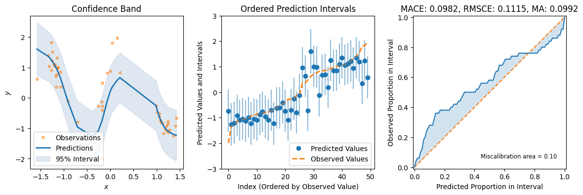
For some additional metrics relevant to UQ, we can use the great uncertainty-toolbox that gives us some insight into the calibration of our prediction. For a discussion of why this is important, see …
[15]:
preds = laplace_model.predict_step(X_test)
fig = plot_calibration_uq_toolbox(
    preds["pred"].cpu().numpy(),
    preds["pred_uct"].numpy(),
    Y_test.cpu().numpy(),
    X_test.cpu().numpy(),
)
Additional Resources#
Daxberger et al. 2020 introduced a subnetwork selection strategy that turns selected weights “Bayesian” while keeping the rest of the network deterministic and show performance on par with deep ensembles.