Quantile Regresssion

%%capture
%pip install git+https://github.com/lightning-uq-box/lightning-uq-box.git

Theoretic Foundation

The goal of Quantile Regression is to extend a standard regression model to also predict conditional quantiles that approximate the true quantiles of the data at hand. It does not make assumptions about the distribution of errors as is usually common. It is a more commonly used method in Econometrics and Time-series forecasting Koeneker, 1978.

In the following we will describe univariate quantile regression. Any chosen conditional quantile \(\alpha \in [0,1]\) can be defined as

\[q_\alpha(x):=\text{inf}\{y \in \mathbb{R}: F(y \vert X = x ) \geq \alpha\},\]

where \(F(y \vert X = x)=P(Y\leq y\vert X = x)\) is a strictly monotonic increasing cumulative density function.

For Quantile Regression, the NN \(f_{\theta}\) parameterized by \(\theta\), is configured to output the number of quantiles that we want to predict. This means that, if we want to predict \(n\) quantiles \([\alpha_1, ... \alpha_n]\),

\[f_{\theta}(x_{\star}) = (\hat{y}_1(x^{\star}), ...,\hat{y}_n(x^{\star})).\]

The model is trained by minimizing the pinball loss function Koeneker, 1978, given by the following loss objective,

\[\mathcal{L}_i (\theta, (x^{\star}, y^{\star})) = \max\{ (1-\alpha_i) (y^{\star}-\hat{y}_i(x^{\star})), \alpha (y^{\star}-\hat{y}_i(x^{\star}))\}.\]

Here \(i \in \{1, ...,n\}\) denotes the number of the quantile and $100:nbsphinx-math:alpha_i $ is the percentage of the quantile for \(\alpha_i \in [0,1)\). Note that for \(\alpha = 1/2\) one recovers the \(\ell^1\) loss.

For an explanation of the pinball loss function you can checkout this blog post.

During inference, the model will output an estimate for your chosen quantiles and these can be used as an indication of aleatoric uncertainty.

Imports

import os
import tempfile
from functools import partial

import matplotlib.pyplot as plt
import numpy as np
import torch
import torch.nn as nn
from lightning import Trainer
from lightning.pytorch import seed_everything
from lightning.pytorch.loggers import CSVLogger

from lightning_uq_box.datamodules import ToyHeteroscedasticDatamodule
from lightning_uq_box.models import MLP
from lightning_uq_box.uq_methods import QuantileRegression
from lightning_uq_box.viz_utils import (
    plot_calibration_uq_toolbox,
    plot_predictions_regression,
    plot_toy_regression_data,
    plot_training_metrics,
)

plt.rcParams["figure.figsize"] = [14, 5]

INFO:root:Asdfghjkl backend not available since the old asdfghjkl dependency is not installed. If you want to use it, run: pip install git+https://git@github.com/wiseodd/asdl@asdfghjkl

seed_everything(0)  # seed everything for reproducibility

Seed set to 0

0

We define a temporary directory to look at some training metrics and results.

my_temp_dir = tempfile.mkdtemp()

Datamodule

To demonstrate the method, we will make use of a Toy Regression Example that is defined as a Lightning Datamodule. While this might seem like overkill for a small toy problem, we think it is more helpful how the individual pieces of the library fit together so you can train models on more complex tasks.

dm = ToyHeteroscedasticDatamodule()

X_train, Y_train, train_loader, X_test, Y_test, test_loader, X_gtext, Y_gtext = (
    dm.X_train,
    dm.Y_train,
    dm.train_dataloader(),
    dm.X_test,
    dm.Y_test,
    dm.test_dataloader(),
    dm.X_gtext,
    dm.Y_gtext,
)

fig = plot_toy_regression_data(X_train, Y_train, X_test, Y_test)

Model

For our Toy Regression problem, we will use a simple Multi-layer Perceptron (MLP) that you can configure to your needs. For the documentation of the MLP see here. For quantile regression we need a network output for each of the quantiles that we want to predict.

quantiles = [0.1, 0.5, 0.9]
network = MLP(
    n_inputs=1, n_hidden=[50, 50, 50], n_outputs=len(quantiles), activation_fn=nn.Tanh()
)
network

MLP(
  (model): Sequential(
    (0): Linear(in_features=1, out_features=50, bias=True)
    (1): Tanh()
    (2): Dropout(p=0.0, inplace=False)
    (3): Linear(in_features=50, out_features=50, bias=True)
    (4): Tanh()
    (5): Dropout(p=0.0, inplace=False)
    (6): Linear(in_features=50, out_features=50, bias=True)
    (7): Tanh()
    (8): Dropout(p=0.0, inplace=False)
    (9): Linear(in_features=50, out_features=3, bias=True)
  )
)

With an underlying neural network, we can now use our desired UQ-Method as a sort of wrapper. All UQ-Methods are implemented as LightningModule that allow us to concisely organize the code and remove as much boilerplate code as possible.

qr_model = QuantileRegression(
    model=network, optimizer=partial(torch.optim.Adam, lr=4e-3), quantiles=quantiles
)

Trainer

Now that we have a LightningDataModule and a UQ-Method as a LightningModule, we can conduct training with a Lightning Trainer. It has tons of options to make your life easier, so we encourage you to check the documentation.

logger = CSVLogger(my_temp_dir)
trainer = Trainer(
    max_epochs=250,  # number of epochs we want to train
    logger=logger,  # log training metrics for later evaluation
    log_every_n_steps=1,
    enable_checkpointing=False,
    enable_progress_bar=False,
    default_root_dir=my_temp_dir,
)

GPU available: False, used: False
TPU available: False, using: 0 TPU cores
HPU available: False, using: 0 HPUs

Training our model is now easy:

trainer.fit(qr_model, dm)

  | Name          | Type             | Params | Mode
-----------------------------------------------------------
0 | model         | MLP              | 5.4 K  | train
1 | loss_fn       | PinballLoss      | 0      | train
2 | train_metrics | MetricCollection | 0      | train
3 | val_metrics   | MetricCollection | 0      | train
4 | test_metrics  | MetricCollection | 0      | train
-----------------------------------------------------------
5.4 K     Trainable params
0         Non-trainable params
5.4 K     Total params
0.021     Total estimated model params size (MB)
23        Modules in train mode
0         Modules in eval mode
`Trainer.fit` stopped: `max_epochs=250` reached.

Training Metrics

To get some insights into how the training went, we can use the utility function to plot the training loss and RMSE metric.

fig = plot_training_metrics(
    os.path.join(my_temp_dir, "lightning_logs"), ["train_loss", "trainRMSE"]
)

Evaluate Predictions

The constructed Data Module contains two possible test variable. X_test are IID samples from the same noise distribution as the training data, while X_gtext (“X ground truth extended”) are dense inputs from the underlying “ground truth” function without any noise that also extends the input range to either side, so we can visualize the method’s UQ tendencies when extrapolating beyond the training data range. Thus, we will use X_gtext for visualization purposes, but use X_test to compute uncertainty and calibration metrics because we want to analyse how well the method has learned the noisy data distribution.

preds = qr_model.predict_step(X_gtext)

fig = plot_predictions_regression(
    X_train,
    Y_train,
    X_gtext,
    Y_gtext,
    preds["pred"],
    pred_quantiles=np.stack(
        [
            preds["lower_quant"],
            preds["pred"].squeeze().cpu().numpy(),
            preds["upper_quant"],
        ],
        axis=-1,
    ),
    aleatoric=preds["aleatoric_uct"],
    title="Quantile Regression",
)

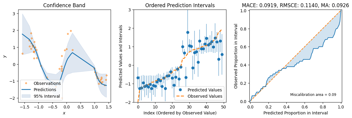
For some additional metrics relevant to UQ, we can use the great uncertainty-toolbox that gives us some insight into the calibration of our prediction.

preds = qr_model.predict_step(X_test)
fig = plot_calibration_uq_toolbox(
    preds["pred"].cpu().numpy(),
    preds["pred_uct"].numpy(),
    Y_test.cpu().numpy(),
    X_test.cpu().numpy(),
)