ZigZag: Universal Sampling-free Uncertainty Estimation#
ZigZag was proposed by Durasov et al 2024.
The work does several evaluations regarding OOD tasks and regards their methods to adress the two types of uncertainty as follows:
“In other words, there are two scenarios when reconstruction fails: 1) when (x, y) is OOD because x is OOD, addressing epistemic uncertainty and OOD samples, 2) when (x, y) is OOD because y is OOD / errornous. In this case, the reconstruction issue is due to y, our uncertainty measure is high, we cover aleatoric uncertainty connected to predicted target.”
Imports#
[1]:
import os
import tempfile
from functools import partial

import matplotlib.pyplot as plt
import torch.nn as nn
from lightning import Trainer
from lightning.pytorch import seed_everything
from lightning.pytorch.loggers import CSVLogger
from torch.optim import Adam

from lightning_uq_box.datamodules import ToyHeteroscedasticDatamodule
from lightning_uq_box.models import MLP
from lightning_uq_box.uq_methods import ZigZagRegression
from lightning_uq_box.viz_utils import (
    plot_calibration_uq_toolbox,
    plot_predictions_regression,
    plot_toy_regression_data,
    plot_training_metrics,
)

plt.rcParams["figure.figsize"] = [14, 5]
INFO:root:Asdfghjkl backend not available since the old asdfghjkl dependency is not installed. If you want to use it, run: pip install git+https://git@github.com/wiseodd/asdl@asdfghjkl
[2]:
seed_everything(0) # seed everything for reproducibility
Seed set to 0
[2]:
0
[3]:
my_temp_dir = tempfile.mkdtemp()
Datamodule#
[4]:
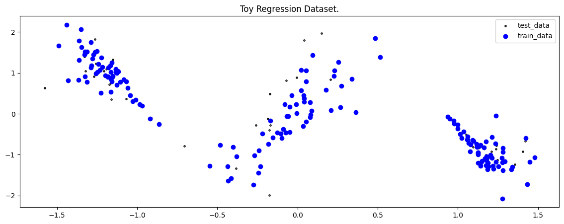
dm = ToyHeteroscedasticDatamodule(batch_size=64)

X_train, Y_train, train_loader, X_test, Y_test, test_loader, X_gtext, Y_gtext = (
    dm.X_train,
    dm.Y_train,
    dm.train_dataloader(),
    dm.X_test,
    dm.Y_test,
    dm.test_dataloader(),
    dm.X_gtext,
    dm.Y_gtext,
)
[5]:
fig = plot_toy_regression_data(X_train, Y_train, X_test, Y_test)
Model#
Here we are creating a deterministic MLP, with two inputs because the ZigZag method is first trained to reconstruct the input and later uses a two-step prediction forward pass, where the features of the first forward pass are concatenated to the original input.
[6]:
network = MLP(n_inputs=2, n_hidden=[50, 50, 50], n_outputs=1, activation_fn=nn.Tanh())
network
[6]:
MLP(
  (model): Sequential(
    (0): Linear(in_features=2, out_features=50, bias=True)
    (1): Tanh()
    (2): Dropout(p=0.0, inplace=False)
    (3): Linear(in_features=50, out_features=50, bias=True)
    (4): Tanh()
    (5): Dropout(p=0.0, inplace=False)
    (6): Linear(in_features=50, out_features=50, bias=True)
    (7): Tanh()
    (8): Dropout(p=0.0, inplace=False)
    (9): Linear(in_features=50, out_features=1, bias=True)
  )
)
When initializing the Masksemble Module, the init will convert the model into a Maskesemble by replacing the layers with Masked Ensemble Layers.
[7]:
zigzag = ZigZagRegression(
    model=network, loss_fn=nn.MSELoss(), optimizer=partial(Adam, lr=3e-3)
)
Trainer#
[8]:
logger = CSVLogger(my_temp_dir)
trainer = Trainer(
    max_epochs=500,  # number of epochs we want to train
    logger=logger,  # log training metrics for later evaluation
    log_every_n_steps=1,
    enable_checkpointing=False,
    enable_progress_bar=False,
    default_root_dir=my_temp_dir,
)
GPU available: False, used: False
TPU available: False, using: 0 TPU cores
HPU available: False, using: 0 HPUs
[9]:
trainer.fit(zigzag, dm)
  | Name          | Type             | Params | Mode
-----------------------------------------------------------
0 | model         | MLP              | 5.3 K  | train
1 | loss_fn       | MSELoss          | 0      | train
2 | train_metrics | MetricCollection | 0      | train
3 | val_metrics   | MetricCollection | 0      | train
4 | test_metrics  | MetricCollection | 0      | train
-----------------------------------------------------------
5.3 K     Trainable params
0         Non-trainable params
5.3 K     Total params
0.021     Total estimated model params size (MB)
23        Modules in train mode
0         Modules in eval mode
`Trainer.fit` stopped: `max_epochs=500` reached.
Training Metrics#
[10]:
fig = plot_training_metrics(
    os.path.join(my_temp_dir, "lightning_logs"), ["train_loss", "trainRMSE"]
)

Prediction#
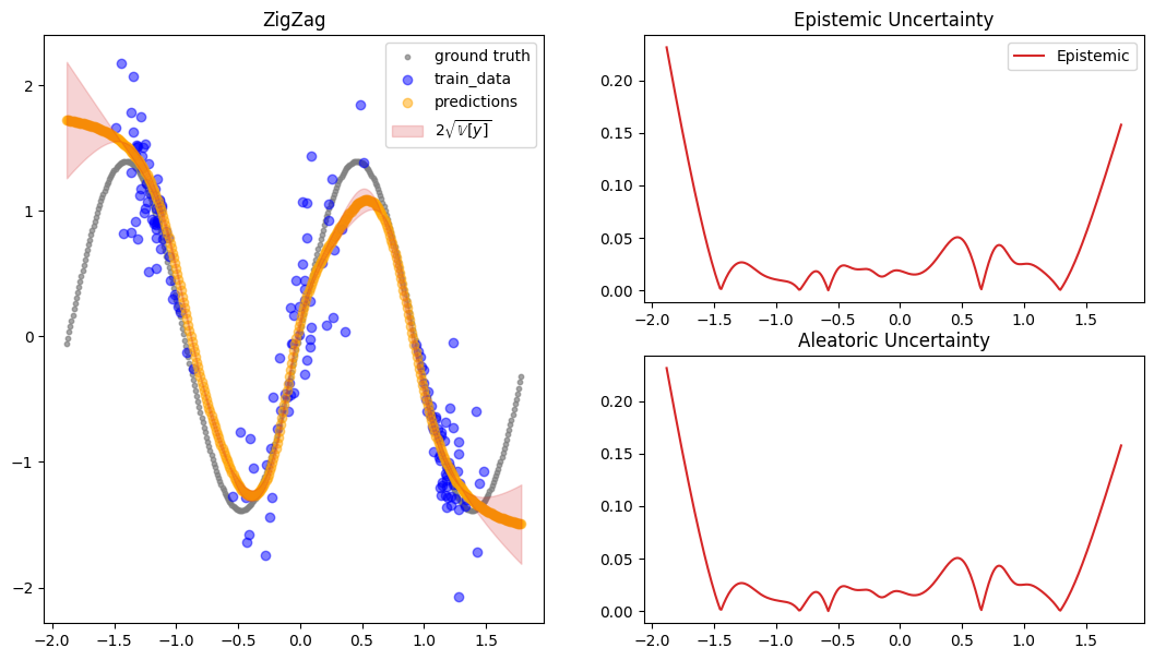
The constructed Data Module contains two possible test variable. X_test are IID samples from the same noise distribution as the training data, while X_gtext (“X ground truth extended”) are dense inputs from the underlying “ground truth” function without any noise that also extends the input range to either side, so we can visualize the method’s UQ tendencies when extrapolating beyond the training data range. Thus, we will use X_gtext for visualization purposes, but use X_test to
compute uncertainty and calibration metrics because we want to analyse how well the method has learned the noisy data distribution.
We visualize the predictive uncertainty as both the epistemic and aleatoric uncertainty because the interpretation depends on inputs and targets as quoted in the beginning.
[11]:
preds = zigzag.predict_step(X_gtext)
fig = plot_predictions_regression(
    X_train,
    Y_train,
    X_gtext,
    Y_gtext,
    preds["pred"],
    preds["pred_uct"],
    epistemic=preds["pred_uct"],
    aleatoric=preds["pred_uct"],
    title="ZigZag",
    show_bands=False,
)
INFO:matplotlib.mathtext:Substituting symbol V from STIXNonUnicode
INFO:matplotlib.mathtext:Substituting symbol V from STIXNonUnicode
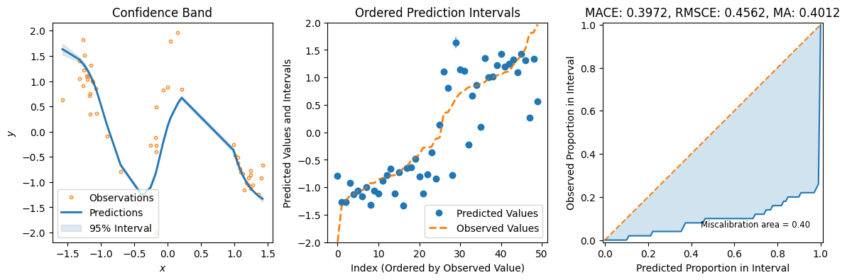
[12]:
preds = zigzag.predict_step(X_test)
fig = plot_calibration_uq_toolbox(
    preds["pred"].cpu().numpy(),
    preds["pred_uct"].cpu().numpy(),
    Y_test.cpu().numpy(),
    X_test.cpu().numpy(),
)
[ ]: