Bayes By Backprop - Mean Field Variational Inference

Theoretic Foundation

Bayesian Neural Networks (BNNs) with variational inference (VI) are an approximate Bayesian method. Here we use the mean-field assumption meaning that the variational distribution can be factorized as a product of individual Gaussian distributions. This method maximizes the evidence lower bound (ELBO) via standard stochastic gradient descent by using the reparameterization trick Kingma, 2013 to backpropagate through the necessary sampling procedure. This results in a diagonal Gaussian approximation of the posterior distribution over the model parameters.

The predictive likelihood is given by,

\[p(Y |\theta ,X) = \prod_{i=1}^K p(y_i|\theta,x_i) = \prod_{i=1}^K \mathcal{N}(y_{i} | f_{\theta}(x_i), \Sigma).\]

The prior on the weights is given by,

\[p(\theta) = \prod_{l=1}^L \prod_{h=1}^{V_l }\prod_{j=1}^{V_{l-1}+1} \mathcal{N}(w_{hj, l} \vert 0, \lambda)\]

where \(w_{hj, l}\) is the h-th row and the j-th column of weight matrix \(\theta_L\) at layer index \(L\) and \(\lambda\) is the prior variance. Note that as we use partially stochastic networks, the above may contain less factors \(\mathcal{N}(w_{hj, l} \vert 0, \lambda)\) depending on how many layers are stochastic. Then, the posterior distribution of the weights is obtained by Bayes’ rule as

\[p(\theta|\mathcal{D}) = \frac{p(Y |\theta ,X) p(\theta)}{p(Y | X)}.\]

As the posterior distribution over the weights is intractable we use a variational approximation,

\[q(\theta) \approx p(\theta|\mathcal{D}),\]

that is a diagonal Gaussian. Now given an input \(x^{\star}\), the predictive distribution can be obtained as

\[p(y^{\star}|x^{\star},\mathcal{D}) = \int p(y^{\star} |\theta , x^{\star}) p(\theta|\mathcal{D}) d\theta.\]

As the above integral is intractable we approximate by sampling form the approximation \(q(\theta)\) to the posterior distribution of the weights. The weights are obtained by minimizing the evidence lower bound (ELBO) on the Kullback-Leibler (KL) divergence between the variational approximation and the posterior distribution over the weights. The ELBO is given by,

\[\mathcal{L}(\theta, (x^{\star}, y^{\star}) ) = \beta D_{KL}(q(\theta) || p(\theta) ) + \frac{1}{2}\text{ln}\left(2\pi\sigma^2\right) + \frac{1}{2\sigma^2}\left(f_{\theta}(x^{\star})-y^{\star}\right)^2 .\]

The KL divergence can be computed analytically as both distributions are assumed to be diagonal Gaussians and the hyperparameter \(\beta\) can be used to weight the influence of the variational parameters relative to that of the data. The hyperparameter \(\sigma\) can be either fixed or set to be an additional output of the network.

The predictive mean is obtained as the mean of the network output \(f_{\theta}\) with \(S\) weight samples from the variational approximation \(\theta_s \sim q(\theta)\),

\[f_m(x^{\star}) = \frac{1}{S} \sum_{s=1}^S f_{\theta_s}(x^{\star}).\]

The predictive uncertainty is given by the standard deviation thereof,

\[\sigma_p(x^{\star}) = \sqrt{\frac{1}{S} \sum_{s=1}^S \left(f_{\theta_s}(x^{\star})- f_m(x^{\star}) \right)^2}.\]

If one uses the NLL and adapts the BNN to output a mean and standard deviation of a Gaussian \(f_{\theta_s}(x^{\star}) = (\mu_{\theta_s}(x^{\star}), \sigma_{\theta_s}(x^{\star}))\), the mean prediction is given by

\[f_m(x^{\star}) = \frac{1}{S} \sum_{s=1}^S \mu_{\theta_s}(x^{\star}).\]

and we obtain the predictive uncertainty as the standard deviation of the corresponding Gaussian mixture model obtained by the weight samples,

\[\sigma_p(x^{\star}) = \sqrt{\frac{1}{S} \sum_{s=1}^S \left(\mu_{\theta_s}(x^{\star})- f_m(x^{\star}) \right)^2+ \sum_{s=1}^S \sigma_{\theta_s}^2(x^{\star})}.\]

%%capture
%pip install git+https://github.com/lightning-uq-box/lightning-uq-box.git

Imports

import os

import tempfile
from functools import partial

import matplotlib.pyplot as plt
import torch
import torch.nn as nn
from lightning import Trainer
from lightning.pytorch import seed_everything
from lightning.pytorch.loggers import CSVLogger

from lightning_uq_box.datamodules import ToyHeteroscedasticDatamodule
from lightning_uq_box.models import MLP
from lightning_uq_box.uq_methods import NLL, BNN_VI_ELBO_Regression
from lightning_uq_box.viz_utils import (
    plot_calibration_uq_toolbox,
    plot_predictions_regression,
    plot_toy_regression_data,
    plot_training_metrics,
)

plt.rcParams["figure.figsize"] = [14, 5]

INFO:root:Asdfghjkl backend not available since the old asdfghjkl dependency is not installed. If you want to use it, run: pip install git+https://git@github.com/wiseodd/asdl@asdfghjkl

seed_everything(0)  # seed everything for reproducibility

Seed set to 0

0

We define a temporary directory to look at some training metrics and results.

my_temp_dir = tempfile.mkdtemp()

Datamodule

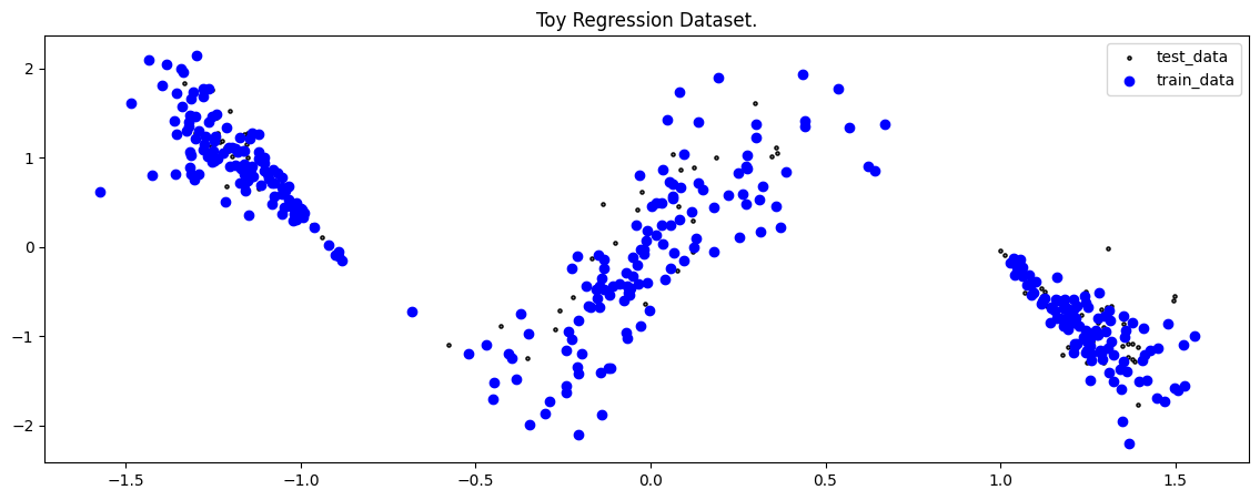
To demonstrate the method, we will make use of a Toy Regression Example that is defined as a Lightning Datamodule. While this might seem like overkill for a small toy problem, we think it is more helpful how the individual pieces of the library fit together so you can train models on more complex tasks.

dm = ToyHeteroscedasticDatamodule(batch_size=32, n_points=500)

X_train, Y_train, train_loader, X_test, Y_test, test_loader, X_gtext, Y_gtext = (
    dm.X_train,
    dm.Y_train,
    dm.train_dataloader(),
    dm.X_test,
    dm.Y_test,
    dm.test_dataloader(),
    dm.X_gtext,
    dm.Y_gtext,
)

fig = plot_toy_regression_data(X_train, Y_train, X_test, Y_test)

Model

For our Toy Regression problem, we will use a simple Multi-layer Perceptron (MLP) that you can configure to your needs. For the documentation of the MLP see here. The following MLP will be converted to a BNN inside the LightningModule.

network = MLP(n_inputs=1, n_hidden=[50, 50], n_outputs=2, activation_fn=nn.ReLU())
network

MLP(
  (model): Sequential(
    (0): Linear(in_features=1, out_features=50, bias=True)
    (1): ReLU()
    (2): Dropout(p=0.0, inplace=False)
    (3): Linear(in_features=50, out_features=50, bias=True)
    (4): ReLU()
    (5): Dropout(p=0.0, inplace=False)
    (6): Linear(in_features=50, out_features=2, bias=True)
  )
)

With an underlying neural network, we can now use our desired UQ-Method as a sort of wrapper. All UQ-Methods are implemented as LightningModule that allow us to concisely organize the code and remove as much boilerplate code as possible.

bbp_model = BNN_VI_ELBO_Regression(
    network,
    optimizer=partial(torch.optim.Adam, lr=3e-3),
    criterion=NLL(),
    stochastic_module_names=[-1],
    num_mc_samples_train=10,
    num_mc_samples_test=25,
    burnin_epochs=20,
)

Trainer

Now that we have a LightningDataModule and a UQ-Method as a LightningModule, we can conduct training with a Lightning Trainer. It has tons of options to make your life easier, so we encourage you to check the documentation.

logger = CSVLogger(my_temp_dir)
trainer = Trainer(
    max_epochs=150,  # number of epochs we want to train
    logger=logger,  # log training metrics for later evaluation
    log_every_n_steps=20,
    enable_checkpointing=False,
    enable_progress_bar=False,
    default_root_dir=my_temp_dir,
)

GPU available: False, used: False
TPU available: False, using: 0 TPU cores
HPU available: False, using: 0 HPUs

Training our model is now easy:

trainer.fit(bbp_model, dm)

  | Name          | Type             | Params | Mode
-----------------------------------------------------------
0 | model         | MLP              | 2.9 K  | train
1 | loss_fn       | NLL              | 0      | train
2 | train_metrics | MetricCollection | 0      | train
3 | val_metrics   | MetricCollection | 0      | train
4 | test_metrics  | MetricCollection | 0      | train
-----------------------------------------------------------
2.9 K     Trainable params
0         Non-trainable params
2.9 K     Total params
0.011     Total estimated model params size (MB)
21        Modules in train mode
0         Modules in eval mode
/home/docs/checkouts/readthedocs.org/user_builds/lightning-uq-box/envs/stable/lib/python3.12/site-packages/lightning/pytorch/loops/fit_loop.py:298: The number of training batches (11) is smaller than the logging interval Trainer(log_every_n_steps=20). Set a lower value for log_every_n_steps if you want to see logs for the training epoch.
`Trainer.fit` stopped: `max_epochs=150` reached.

Training Metrics

To get some insights into how the training went, we can use the utility function to plot the training loss and RMSE metric.

fig = plot_training_metrics(
    os.path.join(my_temp_dir, "lightning_logs"), ["train_loss", "trainRMSE"]
)

Evaluate Predictions

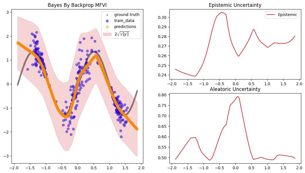
The constructed Data Module contains two possible test variable. X_test are IID samples from the same noise distribution as the training data, while X_gtext (“X ground truth extended”) are dense inputs from the underlying “ground truth” function without any noise that also extends the input range to either side, so we can visualize the method’s UQ tendencies when extrapolating beyond the training data range. Thus, we will use X_gtext for visualization purposes, but use X_test to compute uncertainty and calibration metrics because we want to analyse how well the method has learned the noisy data distribution.

preds = bbp_model.predict_step(X_gtext)

fig = plot_predictions_regression(
    X_train,
    Y_train,
    X_gtext,
    Y_gtext,
    preds["pred"].squeeze(-1),
    preds["pred_uct"],
    epistemic=preds["epistemic_uct"],
    aleatoric=preds["aleatoric_uct"],
    title="Bayes By Backprop MFVI",
    show_bands=False,
)

INFO:matplotlib.mathtext:Substituting symbol V from STIXNonUnicode
INFO:matplotlib.mathtext:Substituting symbol V from STIXNonUnicode

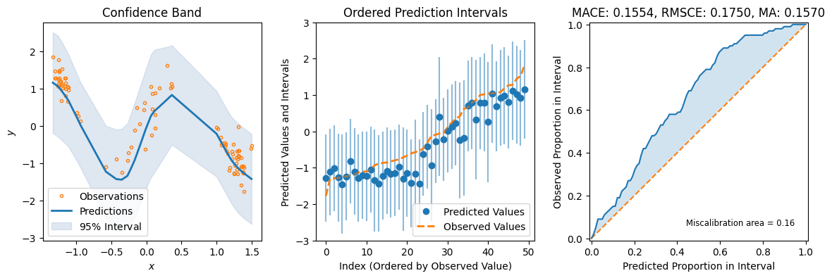
For some additional metrics relevant to UQ, we can use the great uncertainty-toolbox that gives us some insight into the calibration of our prediction. For a discussion of why this is important, see …

preds = bbp_model.predict_step(X_test)
fig = plot_calibration_uq_toolbox(
    preds["pred"].cpu().numpy(),
    preds["pred_uct"].cpu().numpy(),
    Y_test.cpu().numpy(),
    X_test.cpu().numpy(),
)